
Introduction
In this blog post, we will be discussing how to parse a given NetCDF file and how to use the geolocated data to generate an interactive plot with MapLibre.
The data will be sourced from IOOS
Installing Dependencies
Mix.install([
  # Parsing NetCDF files
  {:netcdf, github: "DockYard/netcdf"},
  # Numerical data processing
  {:exla, "~> 0.4"},
  {:maplibre, "~> 0.1"},
  {:kino_maplibre, "~> 0.1", github: "livebook-dev/kino_maplibre"},
  {:req, "~> 0.3.0"}
])

Nx.default_backend(EXLA.Backend)
Obtaining the Dataset
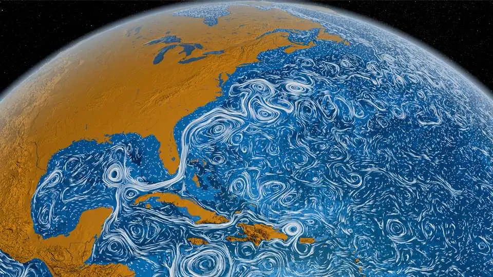
Before we can work on the data, we need to obtain the dataset and parse it. In this post, we are going to process sea current data represented in a NetCDF file format.
To obtain the dataset, we can use the following command:
ncks -p http://edsdata.oceansmap.com/thredds/dodsC/EDS/FVCOM_MASS fvcom_mass20221020.nc ./dataset.nc
This command uses the ncks program, which you will already need to install following the instructions on our NetCDF NIF bindings README to compile the netcdf library correctly. It downloads the data for 2022-10-20 into dataset.nc, which is the path to the destination file.
{:ok, file} = NetCDF.File.open(# path to the NetCDF dataset)
Parsing the dataset into GeoJSON
GeoJSON is a format that represents geolocated data, which MapLibre accepts as input for markers on the map. We’ll leverage this to plot arrows indicating water current speed and direction.
To process the data we can use the code in the ProcessData module we are creating below.
defmodule ProcessData do
  def load(file) do
    # eastward velocity
    {:ok, u_var} = NetCDF.Variable.load(file, "u")
    # northward velocity
    {:ok, v_var} = NetCDF.Variable.load(file, "v")
    # time
    {:ok, t_var} = NetCDF.Variable.load(file, "time")
    # latitude - latc and lonc index the u and v variables
    {:ok, lat_var} = NetCDF.Variable.load(file, "latc")
    # longitude
    {:ok, lon_var} = NetCDF.Variable.load(file, "lonc")

    %{u: u_var, v: v_var, t: t_var, lat: lat_var, lon: lon_var}
  end
The first function load/1 receives an already open NetCDF.File struct and loads the data for the northward and eastward sea current velocities, as well as the time, latitude, and longitude variables that relate to the current values.
  def abs_and_direction_tensors(u_var, v_var, t_var) do
    time_size = length(t_var.value)
    shape = {time_size, :auto}

    u = Nx.tensor(u_var.value, type: u_var.type) |> Nx.reshape(shape)
    v = Nx.tensor(v_var.value, type: v_var.type) |> Nx.reshape(shape)

    # We want to represent the direction as the angle where 0º is
    # "up" and 90º is "right". This is not the conventional "math"
    # angle, but its complement instead.

    # We can achieve these results by loading (u, v) as imaginary and
    # real parts of a complex number. This provides a way to easily calculate
    # the angles in the way we desire, because we can think of the resulting
    # numbers as vectors in a space where the x coordinate is the vertical axis
    # and the y coordinate is the horizontal axis, lining up with the definition
    # above.

    # This also avoids the issue where `Nx.atan2/2` wraps angles around due to domain
    # restrictions.

    complex_velocity = Nx.complex(v, u)

    speed = Nx.abs(complex_velocity)

    # convert m/s to knots
    speed_kt = Nx.multiply(speed, 1.94384)

    direction_rad = Nx.phase(complex_velocity)

    direction_deg = Nx.multiply(direction_rad, 180 / :math.pi())
    # Wrap the values so that they're constrained between 0º and 360º
    direction_deg =
      Nx.select(Nx.less(direction_deg, 0), Nx.add(direction_deg, 360), direction_deg)

    {speed_kt, direction_deg}
  end
The next function is abs_and_direction_tensors, which builds speed and direction Nx.Tensors from the u, v and time data. The code comments go into more detail on how the conversion is done, but the gist of it is that we can treat u and v as the components for a vector and calculate the absolute value and direction from it.
  def filter_to_bounding_box(
        speed,
        direction_deg,
        lat_var,
        lon_var,
        min_lat,
        max_lat,
        min_lon,
        max_lon
      ) do
    # Filtering the data to keep only the geofence of interest
    lat_t = Nx.tensor(lat_var.value)
    lon_t = Nx.tensor(lon_var.value)

    lat_selector = Nx.logical_and(Nx.greater_equal(lat_t, min_lat), Nx.less_equal(lat_t, max_lat))

    lon_selector = Nx.logical_and(Nx.greater_equal(lon_t, min_lon), Nx.less_equal(lon_t, max_lon))

    coord_selector =
      Nx.logical_and(lat_selector, lon_selector)
      |> Nx.new_axis(0)
      |> Nx.tile([Nx.axis_size(speed, 0), 1])

    nan = Nx.tensor(:nan)
    speed = Nx.select(coord_selector, speed, nan)
    direction_deg = Nx.select(coord_selector, direction_deg, nan)
    lat = Nx.select(coord_selector, lat_t, nan)
    lon = Nx.select(coord_selector, lon_t, nan)

    {speed, direction_deg, lat, lon}
  end
The filter_to_bounding_box function will replace all data which is not contained within the given geofence by NaN.
This helps us filter the results accordingly when going back to Elixir land.
  def convert_to_geojson(speed, direction_deg, lat, lon) do
    # indexing at 51 so we only get the time slice at
    # 2022-11-17 00:00:00 @ GMT-3, which was used as
    # a reference
    features =
        [
          Nx.to_flat_list(direction_deg[51]),
          Nx.to_flat_list(speed[51]),
          Nx.to_flat_list(lat),
          Nx.to_flat_list(lon)
        ]
        |> Enum.zip_with(fn
          [:nan | _] ->
            # if one is nan all are nan
            nil

          [direction, speed, lat, lon] ->
            %{
              type: "Feature",
              geometry: %{
                type: "Point",
                coordinates: [lon, lat]
              },
              properties: %{speed: speed, direction: direction}
            }
        end)
        |> Enum.filter(& &1)

    %{type: "FeatureCollection", features: features}
  end
Finally, the last block we need to discuss is the convert_to_geojson function, which receives the previously calculated data and outputs a map in the GeoJSON format which can be fed into MapLibre afterward. This GeoJSON data contains the direction and speed at a given time instant, longitude, and latitude. We offset by 90 degrees because the arrow sprite we are using is oriented pointing to the right. This offset corrects it so that it points upwards at 0 degrees.
  def parse_file_to_geojson(filename, min_lat, max_lat, min_lon, max_lon) do
    {:ok, file} = NetCDF.File.open(filename)

    file_data = load(file)

    {speed, direction_deg} = abs_and_direction_tensors(file_data.u, file_data.v, file_data.t)

    {speed, direction_deg, lat, lon} =
      filter_to_bounding_box(
        speed,
        direction_deg,
        file_data.lat,
        file_data.lon,
        min_lat,
        max_lat,
        min_lon,
        max_lon
      )

    convert_to_geojson(speed, direction_deg, lat, lon)
  end
end
With all that in hand, the parse_to_file_to_geojson connects all of the functions in a single one, which will output the data within the desired geofence. An optional step value is also used to control the sparsity of the plotted arrows.
Running the Code
min_lat = 40
max_lat = 45
min_lon = -72
max_lon = -68

{geojson_data, time_values} =
  ProcessData.parse_file_to_geojson(
    (#...NetCDF dataset path...,
    min_lat,
    max_lat,
    min_lon,
    max_lon
  )
This will yield the geojson data and the time values that are being used. In the next section, we will analyze the code that uses this data to create our interactive map (which can even change along with the time data!)
Plotting GeoJSON
In the PlotDataOnMap module below, we will plot the previous data in a way that renders arrows onto an interactive MapLibre map.
The code is pretty straightforward. First, we read the arrow sprite into memory and then encode it as a data URL string, so it can be fed into an argument that expects an image URL.
Then, we initialize our MapLibre spec centering into the center of our bounding box. Because we’re rendering with kino_maplibre, we need to provide center and zoom first and then animate the transition to the desired bounding box.
One important aspect is that we load the "water-current-speed" MapLibre source into the :symbol layers, which then are configured to use the arrow as the symbol, and into the :circle layer which only uses the speed and the position for each marker.
All of this yields a MapLibre markers positioned, oriented, and scaled according to our input GeoJSON data.
defmodule PlotDataOnMap do
  def run(geojson_data, min_lon, max_lon, min_lat, max_lat) do
    {:ok, arrow_contents} = File.read(#...arrow image in SDF format...)
    image = "data:image/png;base64," <> Base.encode64(arrow_contents)

    bounds = [min_lon, min_lat, max_lon, max_lat]

    alias MapLibre, as: Ml

    arrow_filter = [">=", ["get", "speed"], 0.05]

    Ml.new(
      style: :street,
      center: {(min_lon + max_lon) / 2, (min_lat + max_lat) / 2},
      zoom: 10
    )
    |> Ml.add_source("water-current-speed",
      type: :geojson,
      data: geojson_data,
      cluster: true,
      cluster_radius: 4,
      cluster_max_zoom: 10,
      cluster_properties: %{
        "cl_speed" => ["max", ["get", "speed"]],
        "cl_direction" => ["+", ["get", "direction"]]
      }
    )
    # for smaller zoom levels, we cluster points so fewer arrows are plotted
    # layout and paint private functions help ensure that the arrows are configured
    # in a similar way for clusters and for individual markers
    |> Ml.add_layer(
      id: "clustered-water-current-speed-arrows",
      type: :symbol,
      filter: ["all", ["has", "cl_speed"], [">", ["get", "cl_speed"], 0]],
      source: "water-current-speed",
      layout: layout(["/", ["get", "cl_direction"], ["get", "point_count"]], 0.085),
      paint: paint("cl_speed")
    )
    |> Ml.add_layer(
      id: "water-current-speed-arrows",
      type: :symbol,
      filter: ["all", arrow_filter, ["!", ["has", "cl_speed"]]],
      source: "water-current-speed",
      layout:
        # For individual arrows, we interpolate the size for lower speeds
        layout(["get", "direction"], [
          "*",
          0.125,
          [
            "interpolate",
            ["linear"],
            ["get", "speed"],
            0.0,
            0.5,
            0.56,
            0.8,
            1.13,
            1.0
          ]
        ]),
      paint: paint("speed")
    )
    # For the smallest non-zero speeds, we plot points instead of arrows
    # 0 speed points are not plotted
    |> Ml.add_layer(
      id: "water-current-speed-dot",
      type: :circle,
      filter: [
        "all",
        ["!", ["has", "cl_speed"]],
        ["!", arrow_filter],
        [">", ["get", "speed"], 0],
        [">=", ["zoom"], 12]
      ],
      source: "water-current-speed",
      paint: %{
        "circle-color" => "blue",
        "circle-radius" => 1
      }
    )
    |> Kino.MapLibre.fit_bounds(bounds)
    |> Kino.MapLibre.add_custom_image("arrow-marker", image, sdf: true)
    |> Kino.MapLibre.new()
  end

  defp layout(icon_rotate_expr, icon_size_expr) do
    %{
      "icon-image" => "arrow-marker",
      "icon-allow-overlap" => ["any", true],
      "icon-rotate" => ["-", icon_rotate_expr, 90],
      "icon-size" => icon_size_expr
    }
  end

  defp paint(speed_field) do
    %{
      "icon-color" => [
        "interpolate",
        ["linear"],
        ["get", speed_field],
        0,
        "blue",
        0.56,
        "cyan",
        1.13,
        "green",
        1.69,
        "yellow",
        2.25,
        "red"
      ]
    }
  end
end
We can also use the following code to output our Kino.MapLibre struct. Returning said struct as the result of a Livebook code cell will display an interactive map cell.
PlotDataOnMap.run(geojson_data, min_lon, max_lon, min_lat, max_lat)
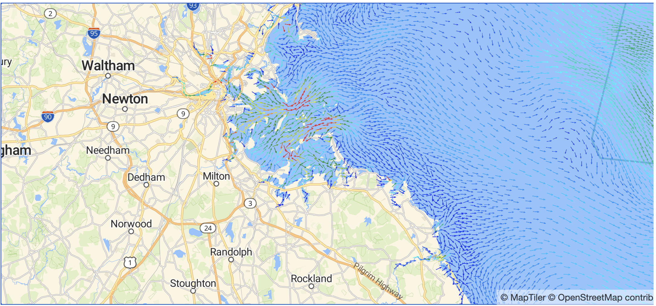
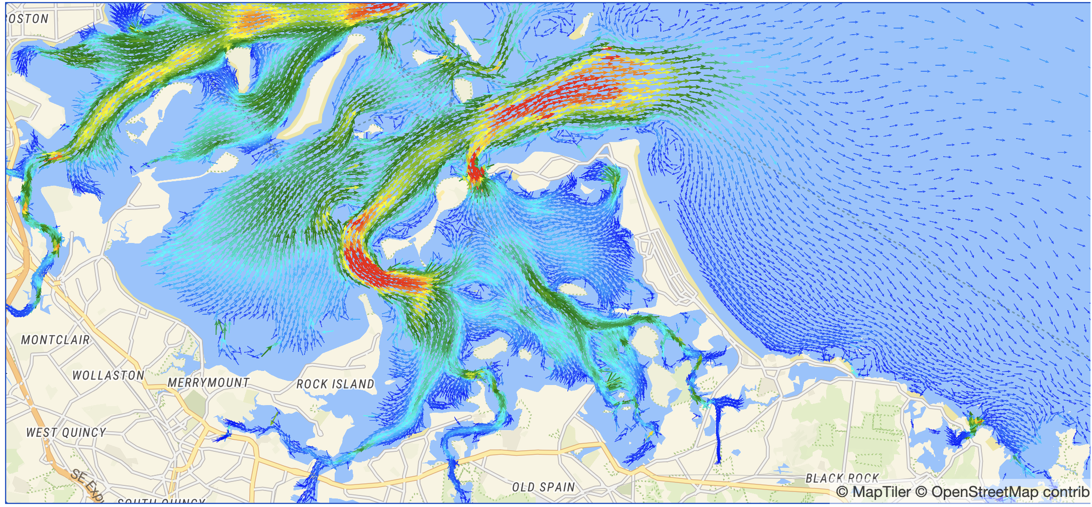
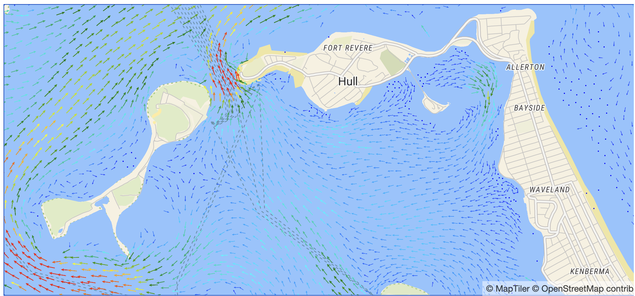
Below, we can see a video and some images of said map cell. They represent the same region in three different zoom levels. From the first to the second image, we also change from clustered markers into individualized markers, which present more information density.
Conclusion
In this blog post, we learned how to parse NetCDF files into Elixir and Nx data structures.
We also learned how to create markers from this data in MapLibre, which helps us visualize the water currents.
It’s important to emphasize that this code currently only works in Livebook because of the dependency on Kino, but the Kino.MapLibre bindings are simple enough that a LiveView version should be easy to put together when needed.
